Abstract
The standard method of refining a macromolecular model uses both automated and manual methods. This combination allows the best abilities of both the computer and the human to be applied to the problem. At a basic level, however, both methods are examining the same indicators of error. This paper discusses some of the properties of these indicators which limit the investigator's ability to identify errors in their models.
Introduction
Our automated refinement packages are limited in that they cannot alter the basic form of the models they are optimizing. Initially the model must be constructed . Interspersed with the automated refinement are sessions of manual intervention. During these sessions at the computer graphics workstation the crystallographic information is presented in the form of density and difference density maps. To properly interpret these maps you must have an understanding of the way errors are represented in these maps and kinds of information not shown by them.
Usually one examines a Fo-Fc map to identify errors in a model and a 2Fo-Fc map to guide the construction of the new model. Since the Fo-Fc map is used to detect the error most of this paper will be devoted to a description of the appearance of these maps.
The first order description of the signal in a Fo-Fc map is know to all crystallographers. Locations in space where there should be electrons show positive features in the map while locations where the model inappropriately contains electrons show negative features. For example, if the model is missing a bound water molecule the Fo-Fc map will show a positive peak at the location where the water molecule should be placed.
A more complicated signal is expected when an atom is modeled but is slightly misplaced. In this case you will expect to see a positive peak next to a negative peak with the atom's current location between. This feature indicates that the atom should be moved toward the positive peak.
These are the signals that all crystallographers are taught to identify. The real situation is more complicated. There are peaks in Fo-Fc maps which do not indicate that atoms should be added to the model and sometimes atoms have errors in their positions which are not marked by pairs of peaks. The proper interpretation of a Fo-Fc map requires that you be familiar with these limitations.
Fo-Fc Map Theory and Limitations
It was shown some time ago (Crukshank, 1951) that least squares minimization and flattening a Fo-Fc map are closely related tasks. This relationship is what allows us to use Fo-Fc map refitting side-by-side with least squares refinement. It was later shown that a relatively simple transformation can convert a Fo-Fc map to the gradient of the least squares' residual (Agarwal, 1978). In fact, this is the way many refinement packages calculate the gradient today. Agarwal's result allows us to treat the Fo-Fc map and the gradient of the least squares' residual function as equivalent.
Therefore, moving atoms to cause the Fo-Fc map to become flat is the same as moving the parameters of the model down the gradient vector. This describes the steepest descent method of function minimization (Leuenberger, 1971). While the steepest descent method is quite robust it is also quite limited.
The principle omission from the steepest descent method is the lack of consideration of any second derivative information. The second derivative of the least squares expression contains several types of information about the model, including
While the Fo-Fc map does not present any second derivative information all refinement packages incorporate some or all of it either directly or indirectly. XPLOR (Brnger, 1987) only includes the second derivative information indirectly via the conjugate gradient procedure (Fletcher and Reeves, 1964, Konnert, 1975). PROLSQ (Hendrickson and Konnert, 1980) uses the precision part (diagonal) of the second derivatives as well as some of the correlation part (off-diagonal) but uses this data ineffectively by using the conjugate gradient method of minimization in roughly the same fashion as XPLOR. TNT (Tronrud, et al, 1987) uses the precision part of the second derivatives with the preconditioned conjugate gradient method (Axelsson, 1985, Tronrud, 1990). While SHELXL (Sheldrick, and Schneider) can use all of the second derivative information the size of the computation required to determine the shift limits its use to small proteins.
The Effect of Parameter Correlation on the Fo-Fc Map
To demonstrate the effect of correlated errors in the parameters of a model I have constructed the following test case.

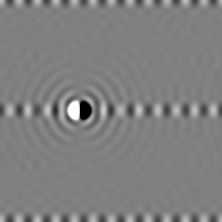
This is one section of a Fo-Fc map. Positive density is white and negative density is black. Regions with no difference density appear neutral gray. The length of each edge is 40. The full unit cell contains 10 atoms, all of which are in their correct position except for the atom in this section which is placed in error by 1.5. While the expected pair of peaks is quite evident there are a considerable number of other features in this section. Despite the complications the pair of peaks are sufficiently clear to indicate the error in the atom's position.
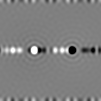
For comparison I have created another Fo-Fc map where I have simply added nine more atoms to the section, each of which are positioned in error by 1.5 in the same direction. In this case there is not a pair of peaks for each atom but a single pair for the entire group of atoms. If you did not consider this group of atoms as a block you would be tempted to simply add a water molecule in the positive peak on the right and increase the B factor of the furthest atom on the left. Since some of the difference density (the three positive peaks on the far right) is fairly strong you might add water molecules there as well. These incorrect modifications of the model would lock the positions of these atoms in the wrong position. This map is very easy to misinterpret.
Since the refinement packages usually do not include second derivative information either they will not usually correct the error in this model either. When there is a concerted shift of a number of atoms you must specifically instruct the refinement package to look for such a shift. However, you will not be able to recognize the existence of this problem from looking at the map and if you perform automated refinement without precautions the computer will make inappropriate shifts and trap your model in error forever.
The lack of consideration of the second derivatives of most refinement packages results in the requirement that you perform rigid body refinement whenever it is possible that your model contains such errors. Usually a model constructed by reference to an m.i.r., s.i.r., or m.a.d. map will not contain errors of this type. However models generated by molecular replacement or molecular substitution (isomorphous mutant or inhibitor structures) often do. In these cases you must perform rigid body refinement with first each entire molecule in a group, then each domain in a rigid group, and perhaps finishing with significant portions of domains defined as rigid groups. Only then can you proceed to individual atom refinement.
You will not see clear indications in your Fo-Fc map that such errors are present even if they are present. To be safe you must perform the rigid body refinement in all cases.
Correlation of Parameters for a Single Atom
While the difference map signals mentioned above, a pair of peaks of opposite sign indicating a positional error and a peak centered on the atom indicating a B factor error, are the form generally taught they are rarely observed in refined difference maps. This is because there is a correlation between the position and B factor of each atom.
If a model is refined and, for some reason, an atom cannot move to accommodate the diffraction data the difference map will develop a pair of peaks. However the atom does not lie halfway between the two peaks - it will be a little closer to the negative peak. Since we have assumed that the atom cannot move to correct the error the only option available to the program is to raise the B factor to attempt to remove the negative peak. By the time the map is examined all that is left to see is a positive peak near an atom. The B factor may be unusually large but that may not be recognizable given the expected fluctuation of this type of parameter.
The most common difference density feature in a refined difference map is positive density near a atom. If there is any density at the position of the atom it is due to restraints preventing the B factor from changing. The response to this density is to search for the restraint which is preventing the atom from moving. If you simply move the atom manually whatever restraint caused the problem will pull the atom back to its original location.
The density of a difference map calculated with an unrefined model will exhibit the classical features.
Series Termination in Fo-Fc Maps
The maps above each contain two principle peaks which indicate the error in position of the group of atoms. Each map also contains a number of other peaks. These peaks are caused by series termination - The lack of certain Fourier terms in the calculation of the maps. All density maps will contain a certain amount of series termination.
The principle cause of series termination is the incompleteness of the observed data set. While the incompleteness of a data set could have many forms usually it is described by an inner (or low) resolution and outer (or high) resolution limit. While the outer resolution limit usually exists because the crystal does not diffract with sufficient intensity to accurately measure (or the structure factors cannot be phased well enough) the inner limit is either chosen arbitrarily or imposed by the technical limitations of the data collection procedure (e.g. the beam stop). The significance of a resolution limit is determined by the amount of intensity lost from the calculation. If the outer resolution limit is caused by the weak diffraction of the crystal at that resolution this limit will not cause significant artifacts in the maps.
If the outer resolution limit is imposed because of phasing errors, as in a m.i.r. map with a breakdown of isomorphism at high resolution, there can be significant series termination errors. In addition the low resolution limit always excludes significant reflections and causes more errors. Since these limits are simple shapes in reciprocal space their effects are simple in real space as well. They cause every feature to be surrounded by ripples. The wavelength of the ripple will be somewhat beyond the resolution limit of the data. For example, a 3 outer resolution limit will cause all features in a map to be surrounded by ripples with a wavelength somewhat shorter than 3. A 6 inner resolution limit will cause ripples somewhat longer than 6.
To demonstrate the affect of series termination on the appearance of a 2Fo-Fc map I will show the results of some model calculations. The z = 0 section of a calculated electron density map for the protein Thermolysin (Holland, et al, 1992) is
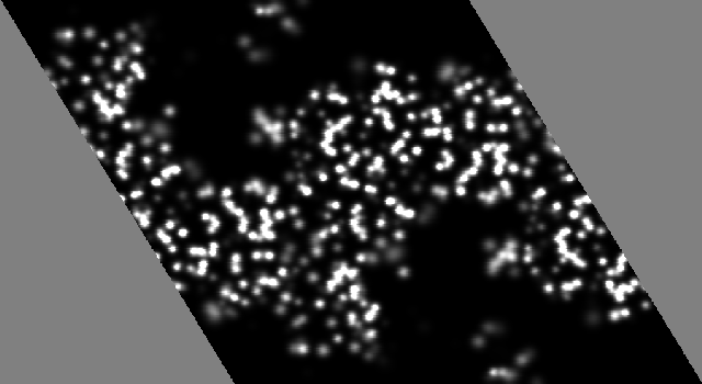
The crystal is hexagonal which explains the gray triangles on the maps sides. Since this map is simply calculated from the atomic positions it does not exhibit any defects due to resolution limits. The bulk solvent regions are devoid of density and the atoms are as resolved as well as can be expected for atoms with B factors of ~15.
A 2Fo-Fc map will never look this good. It will always be missing some of the low resolution data and most likely some of the high resolution data as well. If we recalculate the map shown above with the resolution limits 20 to 1.8 the result is
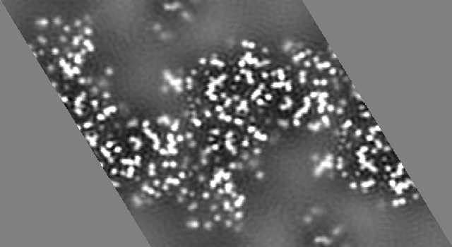
You will note that while the solvent region now appears to contain density the principle features of the protein are still quite recognizable. This map could be used to build a model of the protein without much difficulty.
If the map is calculated again, this time with the resolution limits 6 to 1.8, the result is
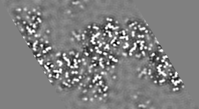
In this map considerable density appears in the bulk solvent regions. While the core of the protein still exhibits sufficient detail to allow the positions of the atoms to be recognized the superposition of the false solvent density on the surface regions of the protein could cause regions with high B factors to be difficult to interpret. In addition there is a great temptation to interpret the "features" in the bulk solvent region as structured solvation.
One must be very cautious when interpreting weak density. There are many explanations for weak features in a map that do not involve the presence of ordered atoms.
Series Termination in Fo-Fc maps
The example shown above mimics a 2Fo-Fc map but series termination also affects Fo-Fc maps. Any error in the protein model will result in features in the Fo-Fc map. These features will be of the classical form - a pair of peaks of opposite sign for positional errors, a peak centered on the atom for a B factor error, and positive density for unmodeled protein - but will be modified by the series termination ripples.
When interpreting a Fo-Fc map you should only attempt to model the strongest features. The weaker features will be distorted by the ripples from the stronger and cannot be reliably interpreted. Once you have corrected the major problems with your model you can calculate a new Fo-Fc map which will show a clearer image of the remaining problems.
Reducing the Parameter Uncertainty
The parameters of your final model will contain uncertainties. These uncertainties arise from the uncertainties in the measurement of the data and are modulated by the mathematical transformation required to calculate the model from those data. Since we do not know how to calculate the model from the data (we can only calculate what the data should be given a model.) the calculation of the uncertainties of our final parameters is quite difficult.
We do know the character of these uncertainties. While we usually talk about the uncertainty of a parameter by estimating a standard deviation, this list of "sigmas" does not tell the whole story. The more troublesome aspect of the uncertainty is the covariance.
The covariance of two parameters quantifies the extent that one parameter can change to compensate for a change in another. Whenever a pair of parameters have a large covariance their values have a much larger uncertainty than their individual standard deviations would indicate.
While it is quite difficult to calculate the covariance of every pair of parameters in a model there are steps which can be taken to reduce the uncertainty. The most powerful is to change the parameters of the model to another set which exhibit less correlation. Usually proteins are modeled by supplying a position and B factor for each atom. When the diffraction data only cover low resolution the parameters for neighboring atoms become highly correlated and their positions quite difficult to refine and their final values quite uncertain. If we knew the basic fold of the protein from some other source (say molecular replacement) we can redefine the parameters of the model. An example of this would be to define the parameters to be the position, orientation, and B factor of each domain in the protein and refine these parameters. Since the electron density of each domain does not overlap the covariance of these parameters will be much smaller.
This example is simply rigid body refinement and is a commonly used means of aiding refinement convergence. While these types of parameter changes are quite powerful current refinement packages are quite limited in their ability to allow parameterizations other than individual atoms and rigid groups.
Usually a new parameterization is devised to make use of some additional source of information. An analogy between the current structure and one solved in another space group provides the information used in the rigid body parameterization. The analogy from one crystal form to another is usually only considered valid at low resolution and the rigid body model is abandoned when refining against high resolution diffraction data.
It would seem reasonable that an analogy between two very similar, isomorphous, structures would be valid to high resolution. If true one could redefine the parameters of the models to be more sensitive to the differences between the two structures. Terwilliger & Berendzen, (1995) have proposed a means of redefining the refinement process to emphasize the differences between the "derivative" and "native" structures (be they mutant verses wild type or inhibited verses uninhibited). While their approach appears promising it does not change the parameterization of either model. The next step would be to define a set of parameters which express the structural details of the two structures in a minimalist form.
Summary
The best source of information about the quality of your model is your maps. If a detail of the structure is not visible in the 2Fo-Fc map and a trial change in this feature of your model does not affect the Fo-Fc map then that detail is probably artifactual. You must be very careful, however, because these maps will contain features which do not arise from the true structure of the protein but are artifacts due to series termination, phase errors, incomplete data, and other sources. To achieve the best maps you must include all available data in their calculation (no omission of the low resolution data) and model all aspects of the structure, including the bulk solvent.
If you are interested in the fine details of your structure you will have to carefully choose the parameters of your model. You should not allow the model to violate facts about the structure such as the conformation of related structures. The parameters of the model should be contrived to allow variability in only those aspects which are believed to differ from known quantities. The fewer parameters the better.
Acknowledgments
This work was supported in part
by NIH grant GM20066 to B. W. Matthews.
Bibliography
Agarwal, R.C., Acta Cryst 34A(1978) 791-809
Axelsson, O., BIT, 25(1985) 166-187
Brnger, A.T., Kuriyan, K., and Karplus, M., Science, 235(1987) 458-460
Crukshank, D., Acta Cryst, 5 (1952) 511-518
Fletcher, R., and Reeves, C., Computer Journal, 7 (1964) 81-84
Hendrickson, W.A., and Konnert, J.H., in Computing in Crystallography, edited by Diamond, R., Ramasechan, S., and Venkatesan, K., 13.01-13.25 (1980), Bangalore: Indian Academy of Sciences
Holland, D.R., Tronrud, D.E., Pleyk, H.W., Flaherty, M., Stark, W., Jansonius, J.N., McKay, D.B., and Matthews, B.W., Biochemistry, 31(1992) 11310-11316
Konnert, J.H., Acta Cryst, 32A(1975) 614-617
Luenberger, D.G., Introduction to Linear and Nonlinear Programming (1973). Reading, MA. Addison-Wesley
Sheldrick, G.M., and Schneider, T.R. in Methods of Enzymology, edited by Sweet, B. and Carter, C., in preparation.
Terwilliger, T.C, and Berendzen, J., 51D (1995) 609-618
Tronrud, D.E., Ten Eyck, L.F., and Matthews, B.W., Acta Cryst, 43A (1987) 489-501
Tronrud, D.E., Acta Cryst, 48A(1992) 912-916